Saturday, September 26, 2020

Towards unification of the four fundamental forces: The Aikyon Theory

SCEST21: Schrodinger's Cat, and Einstein's Space-time, in the 21st Century

A blogspot for discussing the connection between quantum foundations and quantum gravity

Managed by: Tejinder Pal Singh, Physicist, Tata Institute of Fundamental Research, Mumbai

If you are a professional researcher / student researching on these topics, and would like to post an article here with you as author, you are welcome to do so. Please e-mail your write-up to tpsingh@tifr.res.in and it will be uploaded here.


Keywords: Quantum foundations; Quantum gravity; Schrodinger's cat; Spontaneous collapse theory; 
Trace dynamics; Non-commutative geometry; Spontaneous quantum gravity; Classical general relativity; black holes, gyromagnetic ratio 


Saturday, September 26, 2020


Towards unification of the four fundamental forces

https://arxiv.org/abs/2009.05574

https://www.youtube.com/watch?v=uxdvergYNrg&ab_channel=TejinderSingh


The Aikyon Theory


[The word Aikyon derives from `Aikya' in Sanskrit, which means `oneness’. To not make a distinction between space-time and matter].


At the Planck scale, there is no distinction between space-time symmetry and internal symmetry. Physical space is eight dimensional non-commutative octonionic space. One can imagine it as a 2-D complex plane, where the real axis represents 4-D to-be-spacetime, and the imaginary axis represents 4-D to be internal symmetries. The aikyon is an elementary particle, say an electron, *along with* the fields it produces. We do not make a distinction  between the particle and the fields it produces. This is evident from the form of the action for an aikyon, shown below: variables with subscript B stand for the four known forces, and those with subscript F for any of the 24 known fermions of the three generations of the standard model. The Lagrangian is unchanged if B and F variables are interchanged. This is super-symmetry. And since the B-variables include both gravity and gauge-fields, there is a gauge-gravity duality.


The aikyon evolves in this 8-D space in Connes time. The aikyon is a 2D object, as if a membrane [2-brane]. Motion along the real axis is caused by gravity, along vertical axis by electro-colour force, and from real to imaginary by the weak force. Or we can just say, the aikyon moves in the 8D space under the influence of the unified force, given by the  B-variable in the action. 


There is one such action term for every aikyon in this space. Different aikyons interact by `colliding' with each other. The coordinates of this 8D space are the eight components of an octonion. Algebra automorphisms transform one coordinate system to another. These are the analog of general coordinate transformations of general relativity and internal gauge symmetries of gauge theories, and hence unify those concepts. The theory is invariant under 8D algebra automorphisms. And because the laws of motion are those of trace dynamics, this is already a quantum theory.


Saturday, January 11, 2020

Why `quantising' a classical system is like going halfway and then stopping!

SCEST21: Schrodinger's Cat, and Einstein's Space-time, in the 21st Century

A blogspot for discussing the connection between quantum foundations and quantum gravity

Managed by: Tejinder Pal Singh, Physicist, Tata Institute of Fundamental Research, Mumbai

If you are a professional researcher / student researching on these topics, and would like to post an article here with you as author, you are welcome to do so. Please e-mail your write-up to tpsingh@tifr.res.in and it will be uploaded here.


Keywords: Quantum foundations; Quantum gravity; Schrodinger's cat; Spontaneous collapse theory; 
Trace dynamics; Non-commutative geometry; Spontaneous quantum gravity; Classical general relativity; black holes, gyromagnetic ratio 
**********************************


Why `quantising' a classical system is like going halfway and then stopping!

When we quantise a classical system, we raise the canonical variables, q and p, to the status of operators, and assign quantum commutation relations to them: [q, p] = ih

How to recover the classical limit back? It is impossible! One cannot un-quantise a quantised system so as to make it classical again. Because the quantum system obeys linear superposition, and it does so irrespective of the size of the quantum system. Even large quantum systems are demanded by theory to obey superposition, even though they are in fact observed to be classical (no superposition).

The way out of this mess is not that we invent some `interpretation' of quantum mechanics!! The way out is to re-examine how we could have done things differently in the first place.

One very promising way is: ok let us make q and p into operators, but not impose *quantum* commutation relations. The commutation relations are arbitrary, and evolve with time, and are determined by dynamical laws. The dynamical laws are similar to those of classical dynamics, but now adapted to operator variables. This is the theory of Trace Dynamics.

It turns out that for microscopic systems, trace dynamics reduces to quantum theory, quantum commutation relations emerge, and the quantum superposition principle holds. But for large systems, trace dynamics reduces to classical mechanics, and superpositions do not hold [because of the mechanism known as spontaneous localisation, which we discussed earlier].

So, instead of quantising a classical system, one should `operatorise' it: make the commutators arbitrary. Quantisation is like going only half the distance. Trace dynamics is the full story. Thus

Trace Dynamics = Quantum Theory + Spontaneous Localisation.

For small systems, the last bit is negligible. For large systems it is very important.

It is possible to include gravity also in trace dynamics. This leads to a quantum theory of gravity:

Trace Dynamics + Trace Gravity = Quantum gravity + Spontaneous Localisation

For large systems, the last bit is important, and responsible for the emergence of classical space-time and laws of general relativity, from quantum gravity.

Spontaneous Localisation is what un-quantises a quantum system and makes it classical again. Experimentalists are carrying out experiments to find out if spontaneous localisation occurs in nature.

Friday, January 10, 2020

Why does a charged rotating black hole have the same gyromagnetic ratio as an electron?!

SCEST21: Schrodinger's Cat, and Einstein's Space-time, in the 21st Century

A blogspot for discussing the connection between quantum foundations and quantum gravity

Managed by: Tejinder Pal Singh, Physicist, Tata Institute of Fundamental Research, Mumbai

If you are a professional researcher / student researching on these topics, and would like to post an article here with you as author, you are welcome to do so. Please e-mail your write-up to tpsingh@tifr.res.in and it will be uploaded here.


Keywords: Quantum foundations; Quantum gravity; Schrodinger's cat; Spontaneous collapse theory; 

Trace dynamics; Non-commutative geometry; Spontaneous quantum gravity; Classical general relativity 
***************************

January 11, 2020


Why does a charged rotating black hole have the same gyromagnetic ratio as an electron?!


We know that a charge moving in a magnetic field experiences a force. A moving charge is of course a current. So, a current carrying wire experiences a force in a magnetic field. The same would be true if the wire forms a closed loop, say for simplicity a circular loop with some radius, in which a charge is going around with some angular velocity. The response of such a charge to an external magnetic field depends on the value of the charge, the angular speed, and the area of the loop. These quantities combine to define the magnetic moment of the current loop, which is simply current times the area. The response of a current in a loop depends on the magnetic moment, and is essentially magnetic moment times the external magnetic field.

It is easy to show that the magnetic moment is proportional to the orbital angular momentum of the charge in the loop. The ratio of the magnetic moment to the angular momentum is a constant q/2m, independent of the parameters of the orbit, where q is the magnitude of the charge, and m the mass of the particle. This ratio, q/2m, known as the gyromagnetic ratio, is the object of our interest in today’s post.

So if we have an electron with a charge e and mass m going around in a loop, it will have a g-ratio of e/2m. Now, an electron also has a spin, I.e. an intrinsic angular momentum, distinct from orbital angular momentum. It is a purely quantum mechanical effect, arising out of the Dirac equation, and the spin of an electron is one-half the Planck constant. The electron also has an intrinsic magnetic moment because it is a charge with angular momentum. Again, this magnetic moment is proportional to intrinsic angular momentum, but the g-ratio is now e/m, not e/2m. This can be proved from the Dirac equation. The g-ratio of a Dirac fermion is twice the classical value - this can be proved from the Dirac equation. Nothing terribly surprising if the quantum value is twice the classical value. The surprise comes now, when we talk of black holes.

Black holes are solutions of Einstein equations, and their properties are determined by the laws of classical general relativity. These laws are *classical*, not quantum, and black holes are classical objects. A black hole is described by at most three parameters - its mass, charge, and angular momentum, let’s label them M, Q and J respectively. The composition of this mass is not relevant for describing a black hole. Already we see something striking - an electron is also described by its mass, charge, and (spin) angular momentum! A black hole with no charge or angular momentum is described only by its mass M, and is called the Schwarzschild black hole. A Reissner-Nordstrom black hole has mass and charge, but no angular momentum. The most general black hole is the Kerr-Newman black hole, where M, Q and J are all non-zero. This is the charged rotating black hole. It has a magnetic moment, and a g-ratio, which can be calculated from Einstein equations. The g-ratio turns out to be Q/M, not Q/2M, agreeing with the Dirac quantum value for the electron, and disagreeing with the classical value! Even though black holes are classical objects.

This should set alarm bells ringing. In my view, this is a great hint that, despite appearances. Einstein equations have something to do with the Dirac equation, and black holes have something to do with Dirac fermions. Thus, since classical general relativity (with matter) is an approximation to a quantum gravity theory (along with matter), the latter theory must explain why a black hole has a g-ratio twice the classical value. This should be a requirement for a quantum gravity theory to be viable.

There is already considerable evidence in known physics that Einstein equations are deeply connected with the Dirac equation. Firstly, if we ask how to describe the dynamics of a relativistic particle of some mass m, the answer is ambiguous. We could describe it by the Dirac equation, which claims to hold for arbitrary values of mass; or we could describe it by Einstein equations, which also claim to hold for arbitrary values of the mass. Obviously, both descriptions cannot be correct. From experience we know that Dirac equation works for small particles, which are quantum in nature, and Einstein equations work for large objects, which are classical in nature. But how small is small, and how large is large? Neither the Dirac equation nor Einstein equations have  a mass scale. Obviously then, there ought to exist an underlying theory with a mass scale (or equivalently a length scale), such that for masses much smaller than this scale, the theory reduces to Dirac equation for quantum systems. And for masses much larger than this scale, the theory reduces to Einstein equations for classical systems.

The next big hint that Einstein equations are connected with Dirac equations, comes from geometry - something we discussed in an earlier post. Given  a Riemannian manifold, and the standard Dirac operator on it, the sum of the eigenvalues of the square of the Dirac operator is proportional to the Einstein-Hilbert action on this manifold. This remarkable result again suggests an Einstein-Dirac connection, provided we figure out a way to include Dirac fermions in the theory.

This is precisely what has been done in our recently proposed theory of spontaneous quantum gravity. An atom of space-time-matter has an associated length scale L, which is interpreted as its Compton wave length. If L is much larger than Planck length the theory reduces to quantum theory and the Dirac equation for a fermion. If L is much smaller than Planck length, the equations describing the STM atoms reduce to Einstein equations of general relativity, and the collection of STM atoms can be shown to be a classical black hole! One way to understand this is to note that given L, one can define another length from it, namely the square of Planck length divided by L. This is a quantity equal to the Schwarzschild radius, and it exceeds Planck length when L goes below Planck length. Thus when L crosses from a value larger than Planck length to a value smaller than Planck length, there is a cross-over from the Dirac fermion phase to the Einstein black hole phase. The net mass in the system crosses over from less than Planck mass to greater than Planck mass. A collection of entangled STM atoms behaves quantum mechanically, obeying the Dirac equation, if the total mass is less than Planck mass. The collection behaves like a black hole if he total mass exceeds Planck mass.

There in fact is a duality which maps a Dirac fermion to a black hole. It can be shown that if a solution describes an STM atom with Compton wavelength L, the adjoint of this solution describes a black hole with Schwarzschild radius L and Compton length L’=L_P^2/L. Now, if we associate an electric charge e with the Dirac fermion, we can associate a dipole moment eL with the STM atom. There is strong evidence that this dipole moment remains unchanged under the said duality map, which maps the Dirac fermion to a black hole with charge Q and mass M=1/L’ in such a way that eL = QL’. But this product is nothing but the gyromagnetic ratio. Hence this duality between Dirac fermions and black holes explains why a charged rotating black hole has the same gyromagnetic ratio as the electron. Black holes and electrons are simply two different states of atoms of space-time-matter. We consider this to be compelling evidence that spontaneous quantum gravity is a viable theory of quantum gravity.

Brief introduction to Quantum Foundations

SCEST21: Schrodinger's Cat, and Einstein's Space-time, in the 21st Century

A blogspot for discussing the connection between quantum foundations and quantum gravity


If you are a professional researcher / student researching on these topics, and would like to post an article here with you as author, you are welcome to do so. Please e-mail your write-up to tpsingh@tifr.res.in and it will be uploaded here.


Brief Introduction to quantum foundations

Shivnag 
IISc, Bangalore

In this post, I shall attempt to briefly examine some of the foundational issues of quantum mechanics (which I will abbreviate as QM for convenience). I think it is a good idea to remind the well-experienced practitioners of QM every now and then the fact that they don't really understand what they are working with. That is, this post serves to remind us of the fact that QM is, at its heart, quite messed up. On a more pragmatic note, with all the talk about entanglement-this and entanglement-that (every guy on the street who has heard the word “quantum” has probably heard of it attached to the word “entanglement”), it is perhaps a good idea to understand what exactly entanglement is and what's the big deal about it. If you do wish to pursue these issues in more details, you inevitably arrive at the doorstep of quantum computation and quantum information, but that's for a later day (and a later post). So, let's get started!
Setting the Stage
First off, what are the features of quantum mechanics you found most annoying when learning about it in your sophomore (or was it junior) year? Most of us would agree that it was rather unsettling to see that QM answers to questions like “What precise outcome do we observe when we make a measurement?” by giving a set of possible outcomes and telling us the likelihood of each outcome. That is, if you were to perform the same experiment a million times under identical conditions, you could use QM to conclude how many of those times you'd get outcome A or outcome B, or you might be able to say that outcome C is ruled out because it is not in the set of allowed outcomes predicted by QM. While this is progress in itself, it begs the question, “Why can't I predict the precise outcome of any one experiment?” The first thing that we are told in our QM courses is that the problem is qualitatively different from say, the problem with predicting whether you get heads or tails on a coin toss. In principle, you could predict the outcome of a toss if you knew the exact mass distribution of the coin, the exact angular velocity with which it is flipped, the exact pressure distribution of air molecules which create drag on the coin etc. In addition to knowing every last detail about the coin, its surroundings and how you toss it, you'd need to have a computer powerful enough to process all that information (and preferably do it before the coin landed back in your hand). Needless to say, we'll not be discarding our method of using coin tosses to decide who bats first anytime soon. However, what's important is that it can be done.
However, we are told that the situation is different in QM. That is, it isn't a technological limitation that is preventing us from predicting the outcome of a single run of an experiment. The uncertainty is built into the physical laws. That is, no matter how powerful a computer you build, you'll not be able to predict the outcome of a quantum measurement precisely. Naturally, the first question that comes to mind is, “How are we sure that QM is the whole story?” And I am not posing this question in any deep, philosophical sense (that's for later). The most pedestrian objection one can have to this line of thought is, “Isn't it possible that QM is not capable of understanding some interaction (or missing something else) and that's the reason why it fails to predict precise outcomes?” Or one may wonder, “Maybe nature has some additional variables that need to be measured and fed into our mathematical machinery to get precise predictions?” Both these questions are important, and both bothered physicists and philosophers alike over the past century. Also, if the answer to either question is a yes, then that would mean that QM is incomplete or worse, wrong. The latter is unlikely because we have verified the predictions of QM countless times in numerous situations. You are doing it right now as you read this - for instance, QM provides the theoretical framework for understanding and working with the semiconductor electronics which power your computer. However, it surely can be incomplete, and one school of thought is to try and probe (no pun intended!) the question of how measurement works in quantum mechanics. This might not be as futile a venture as people these days make it to be. After all, Einstein arrived at special relativity, by examining the question of how you measure distances and times (that's what led him to conclude that simultaneity is not an absolute concept). The same could be true for quantum mechanics too, because the truth is, we don't have a good idea as to what exactly constitutes a measurement in quantum mechanics.
I will try to make some progress in this direction by trying answer the two questions I posed above. I will start with the second one - that is, the question of whether there are variables in Nature which haven't been observed and which, if observed, could eliminate the uncertainties in quantum mechanics. In fact, Einstein & co. believed that this was indeed the case and the great lengths they went to in order to prove their point is the stuff of legends. The argument that Nature has hidden variables that we have not (or cannot) observe go by the rather unimaginative name of “hidden variable theories”. I will examine their argument in the next post and see how (if at all) this argument can be verified.

Thursday, December 5, 2019

The theory of spontaneous quantum gravity: an overview


SCEST21: Schrodinger's Cat, and Einstein's Space-time, in the 21st Century

A blogspot for discussing the connection between quantum foundations and quantum gravity

Managed by: Tejinder Pal Singh, Physicist, Tata Institute of Fundamental Research, Mumbai

If you are a professional researcher / student researching on these topics, and would like to post an article here with you as author, you are welcome to do so. Please e-mail your write-up to tpsingh@tifr.res.in and it will be uploaded here.


Keywords: Quantum foundations; Quantum gravity; Schrodinger's cat; Spontaneous collapse theory; 

Trace dynamics; Non-commutative geometry; Spontaneous quantum gravity; Classical general relativity 
***************************

December 5, 2019

The theory of Spontaneous Quantum Gravity: an overview

YouTube Video   https://youtu.be/lJk_mE8K8uw

Tejinder Singh

As we have seen in the previous posts, we would like an underlying theory for spontaneous collapse, which also provides  a relativistic description of collapse. Trace dynamics goes a good part of the way, by deriving quantum field theory as the equilibrium statistical mechanics of an underlying matrix dynamics with global unitary invariance. Brownian motion fluctuations about equilibrium can provide the origin of spontaneous localisation, subject to a few assumptions. Trace dynamics operates at the Planck scale, but assumes space-time to be flat Minkowski space-time. Quantum theory is then derived by coarse graining trace dynamics over time scales much larger than Planck time. Quantum dynamics is thus a low energy emergent phenomenon, emerging after this coarse graining. 

It is desirable though that we include gravity in trace dynamics, considering that Planck scale physics is involved. We also recall our other goal to have a formulation of quantum (field) theory without classical space-time. It turns out that the TD formalism can help us do that, if we can find a way to incorporate gravity. This would then also be a theory of quantum gravity. We also emphasised earlier that quantum gravity must dynamically explain the absence of space-time superpositions in the classical limit. That goal will be achieved here, because TD already has a mechanism (fluctuations) to explain spontaneous collapse.

So, how do we bring in gravity? It cannot be brought in simply as classical general relativity. That is not allowed by the Einstein hole argument: the matter in TD is not classical, whereas classical matter fields are needed to give operational meaning to the point structure of classical space-time. We also recall that trace dynamics describes matter degrees of freedom as matrices, which do not commute with each other. We search for a similar matrix/operator type description of gravity, which should not already be tied to quantisation of classical gravity. Because quantum theory should in fact emerge from the sought for [trace dynamics + gravity] after coarse-graining over Planck time scales. Thus we seek a matrix dynamics description of [matter + gravity], on the Planck scale.

Fortunately, such a matrix type description of gravity exists - it is the non-commutative geometry (NCG) program discovered and developed  by Alain Connes and collaborators. From our point of view, keeping trace dynamics in mind, NCG could be introduced as follows: what kind of geometry would we get if we raised space-time points (described by real numbers) to the status of matrices/operators? Recall we did just this kind of thing for material particles and gauge fields in TD. Similarly, our space-time points now become operators, which in general do not commute with each other. 

In a mathematical approach, this can be understood as follows. Physical space, or space-time, is described by the laws of geometry. It can be mapped to an algebra, by assigning coordinates to the points of space. Then geometric properties (such as curvature) can be described in terms of functions on the algebra. This of course is a commutative algebra - real numbers commute with each other. After mapping the geometry of the space to a (commutative) algebra, we now take the following step: we make the algebra non-commutative. This is precisely what is achieved by elevating points of the space (or space-time) to matrices. The matrices do not commute with each other, and hence we have a non-commutative algebra. Now we ask: what kind of geometry such a non-commutative algebra describe?! That `geometry’, we call non-commutative geometry. There is no corresponding geometry in the sense in which we relate geometry to space, but we can talk of analogous concepts: e.g. what is the curvature of a non-commutative space? 

One immediately notices the striking parallel between trace dynamics on the one hand, and NCG on the other. Both obtain by elevating classical point structures to the status of non-commuting operators. The former arrives at a matrix dynamics for matter and gauge fields. The latter arrives at a matrix description of geometry. Now classical general relativity couples classical matter to Riemannian geometry: matter curves space-time. We then expect matter described by trace dynamics to couple to non-commutative geometry: matrix matter `curves’ non-commutative space-time. Thus we intend to built a matrix theory of matter + gravity by unifying trace dynamics with non-commutative geometry. And we demand that this matrix dynamics have the following properties: when we perform the statistical mechanics of this gravity-based matrix dynamics, we should obtain a quantum theory of gravity at equilibrium. Fluctuations should become important for macroscopic systems (macroscopic to be defined) and spontaneous collapse should then come into play, giving rise to an emergent classical space-time and classical matter fields, such that the classical space-time has a Riemannian geometry which obeys the laws of general relativity. Fortunately, a mathematical formalism for such a programme has been developed: this is the theory of Spontaneous Quantum Gravity (SQG). SQG is in fact trace dynamics + trace gravity (i.e. NCG). From here, quantum gravity, quantum (field) theory, and classical general relativity, and classical dynamics, are all emergent phenomena.

What would such a matrix gravity look like, mathematically? Naively, we might want to make coordinates into operators, raise each metric component to an operator, try to construct a curvature tensor operator, and somehow couple it to the trace Lagrangian for matter fields in TD. But this does not work, for various reasons. It is technically difficult to make an invariant four-volume from the determinant of the metric, when each metric component is an operator. It all does not have the right feel, to say the least. Furthermore, classical space-time has been lost; how will we even describe time evolution and hence the dynamics, in matrix gravity? 

Fortunately, the formalism of NCG shows the way forward. One can properly describe concepts such as distance and metric, in a non-commutative geometry. What is very important is that NCG seems to provide a new fundamental time parameter - a property unique to non-commutative geometry, not found in commutative algebras. We will return to this in some detail in future posts - for now we just accept and employ this time parameter, which we will call Connes time. We lost space-time, but we recover time, and that is adequate for dynamics. Time is more fundamental than space.

When we raise space-time points to operators/matrices, like in TD, we can try to use the TD language of Grassmann matrices. In classical GR, metric is a field that lives on space-time. That won’t do now: trying to make something live on an operator. We expect the space-time operator to describe space-time geometry itself, and indeed that does happen. Also, we need to ask - the Grassmann matrix that represents space-time geometry: should it be just bosonic, or should it have a fermionic part too? I don’t at present know he answer to this important question. For now, we work with a Grassmann even (i.e. bosonic) matrix to describe spacetime geometry. 

Since we want matrix gravity to yield GR (with matter sources) in the classical limit, we will have to specify a Lagrangian - both for gravity and for matter. Again, NCG shows the way, for gravity. There is a remarkable result in geometry, which relates curvature in a Riemannian geometry, to the Dirac operator on this space-time. Consider a Riemannian space - having a Euclidean signature. For now, and in this SQG program, we work with the Euclidean case. The Lorentzian case remains to be developed. Given a curved Riemannian space, one can write the standard Dirac operator DB on it [`gamma-mu del-mu’] in terms of the gamma-matrices and the spatial derivatives. A result from geometry states that [expressed for now as a simplified statement] the trace of the square of the Dirac operator is equal to the Einstein-Hilbert action [`integral of R root(g)’]. Isn’t that surprising - that the sum of the eigenvalues of the Dirac operator on a space is connected to Riemannian curvature on that space. The eigenvalues of the Dirac operator are connected to gravity - in fact they *are* gravity, as we will see later. The metric can be connected to these eigenvalues. 

So we have this operator, DB2 on a Riemannian space. We can make the algebra of coordinates non-commutative, and we will still have this square of the Dirac operator: it describes curvature on a non-commutative space. And we nave the Connes time, labelled say tau, to describe evolution. We can now make contact with trace dynamics; recall that the trace Lagrangian is trace of an operator polynomial in configuration variables and their velocities. The trace polynomial coming from NCG is trace of square of the Dirac operator. Remembering that in quantum mechanics the Dirac operator is like momentum, we now introduce in our theory a bosonic operator/matrix qB such that its derivative with respect to Connes time is the Dirac operator DB. This is the defining condition for qB while the defining condition for the Dirac operator is as before: it becomes the ordinary Dirac operator on a Riemannian space, and there it relates to the Ricci scalar and the Einstein-Hilbert action. In matrix gravity, the action describing gravity is the (Connes) time integral of the trace of the squared Dirac operator. This has just the form expected from trace dynamics. Moreover, the Lagrange equation resulting from this action is also very simple: the momentum is constant in time, and the configuration variable evolves linearly with time.

Next, we must include matter, because we after all want to derive spontaneous localisation of matter, from the SQG theory. At this stage in this programme we consider matter fermions only, leaving the consideration of (bosonic) gauge fields and non-gravitational interactions for later. So we have to have a way to include say Dirac fermions, in the language of trace dynamics. One thing we can anticipate is that these will be described by fermionic Grassmann matrices. But what should the Lagrangian be, keeping also in mind that we also have the Dirac operator at hand. We could construct a trace Lagrangian for every fermion in the theory, add up these Lagrangians, and add this to the trace Lagrangian for gravity (described above), integrate it over Connes time, and that could give the action for matrix dynamics. 

However, we do not go on that path, for conceptual reasons. Let us ask the question: what is the gravitational  effect of an electron? An electron, being quantum mechanical, is all over space; so why must we distinguish the gravitational effect of the electron from the electron itself? This situation is unlike that of a classical object, say planet earth, where the object is localised in space, and its gravitational field is spread out everywhere. So we propose to introduce the concept of an `atom’ of space-time-matter [STM] which is a combined description of the fermionic part (say the electron) to be described by a fermionic operator qF, and its gravitation part, to  be described by the bosonic qB. Thus, we define the operator q for an STM atom, written in terms of its bosonic and fermionic parts: q = qB + qF. For instance, in matrix gravity, an electron along with its gravity is an STM atom - it comes with its own operator space-time coordinates, its own Dirac operator. Further, we define the fermionic part of the Dirac operator, DF to be the Connes time derivative of qF. And the full Dirac operator D by D = DB + DF. Recall that the original Dirac operator DB is bosonic. The Lagrangian for an STM atom is the trace of the square of D, and the action is the time integral of this Lagrangian. There is one such term for each STM atom. We can write the total action for matrix gravity simply as: 


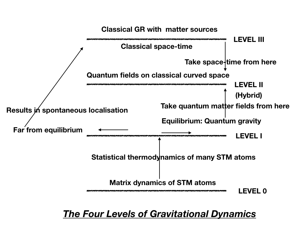
This is nice. From here we can derive quantum gravity, quantum theory, classical general relativity, all as emergent phenomena. To begin with, one easily obtains the Lagrange equations for the bosonic and fermionic part of each STM atom. The momenta are constant, and the configuration variables evolve linearly with time. Because of unitary invariance, there again is a conserved Adler-Millard charge. The following diagram helps us understand where to go next.  


What we have described so far takes place at Level 0. There are only two fundamental constants at Level 0 - Planck length and Planck time. And there is the conserved Adler-Millard charge. Every STM atom has only one associated parameter, a length scale L, which eventually gets interpreted as Compton wavelength (L can be different for every atom). At Level 0,  there is no Planck’s constant, no Newton’s gravitational constant, no concept of mass nor spin: all these are emergent at higher levels. At level 0, there is only the length scale L, from which mass and spin emerge subsequently at Level I. How do the STM atoms interact with each other? `Collisions’ and entanglement are possible mechanisms - this aspect is currently under investigation.

Level 0 is a Hilbert space on which the operators describing STM atoms live, and evolve in Connes time. Dynamics take place at the Planck scale, as in trace dynamics. There is no space-time here. Space-time and the laws of general relativity emerge at Level III, as a consequence of spontaneous localisation. We can say that space-time arises as a consequence of collapse of the wave-function; more specifically, the part of the wave function that describes the fermions. The bosonic part does not undergo localisation, and becomes space-time and its curvature.

Like in trace dynamics, we would like to know what the emergent dynamics at low energies is, if we average Level 0 dynamics over time scales much larger than Planck time. For this we perform the statistical thermodynamics of the STM atoms described by the action given in the equation above. What emerges, at equilibrium at Level I, are the standard quantum commutation relations, and Heisenberg equations of motion, separately for the bosonic and fermionic parts of each STM atom. Evolution is still in Connes time. Planck’s constant emerges too, and hence Newton’s gravitational constant can be defined, using Planck’s constant along with Planck time and Planck length. The mass of an STM atom is defined in terms of its length L, which length hence can be interpreted as its Compton wavelength. The Schwarzschild radius of an STM atom is defined as square of Planck length divided by L. One can transform to the Schrodinger picture dynamics as well, and define quantum entanglement. Thus what we have at equilibrium at Level I is a quantum theory of gravity, emergent from the Level 0 matrix gravity dynamics. If we would like to know what is the gravitation of an electron, we can answer that question at Level I, or at Level 0, but not at Level II or III. Note that this Level I quantum gravity is a low energy phenomenon! It does not have anything to do with the Planck scale, but rather comes into play whenever a background space-time is not available. This Level I quantum gravity is also the sought after description of quantum (field) theory without classical time.

If a sufficiently large number of STM atoms get entangled, something very interesting takes place. If the total mass of the entangled system of STM atoms goes above Planck mass, the effective Compton wavelength of the full system goes below Planck length. The approximation that we can coarse grain the Level 0 dynamics over times larger than  Planck times breaks down. This is what we mean by fluctuations becoming important. The entangled system experiences rapid Planck scale fluctuations, an anti-self-adjoint part from the fermionic trace Hamiltonian is no longer negligible, and the entangled system undergoes extremely rapid spontaneous localisation. The localisation of the fermionic parts of many such entangled systems gives rise to the macroscopic bodies of the universe. Their bosonic parts together describe classical gravity, which is shown to obey the laws of classical general relativity. 


Those STM atoms which do not undergo spontaneous localisation are to be described at Level 0 or Level I. Or, if we neglect their gravity, we can describe them at the hybrid Level II, after borrowing the space-time part from Level III. This is how we  conventionally do quantum (field) theory.

The theory of Spontaneous Quantum Gravity makes the following predictions:

1. Spontaneous localisation (the GRW theory) is a prediction of this  theory, and the GRW theory is being tested in labs currently. If the GRW theory is ruled out by experiments, this proposal will be ruled out too.

2. SQG predicts the novel phenomena of quantum interference in time, and spontaneous collapse in time. 

3.The theory predicts the Karolyhazy length as a minimum length. This is testable and falsifiable.

4. This theory predicts that dark energy is a quantum gravitational phenomenon.

5. The theory provides an explanation for black hole entropy, from the microstates of STM atoms.

In forthcoming posts, we will discuss the SQG theory as well as its predictions in some detail. SQG is a candidate cover theory for general relativity, in the sense discussed in the first post. It explains the emergence of the classical world from quantum gravity, without having to resort to any interpretation of quantum mechanics.


Tuesday, December 3, 2019

The origin of spontaneous localisation: Trace Dynamics III


SCEST21: Schrodinger's Cat, and Einstein's Space-time, in the 21st Century

A blogspot for discussing the connection between quantum foundations and quantum gravity

Managed by: Tejinder Pal Singh, Physicist, Tata Institute of Fundamental Research, Mumbai

If you are a professional researcher / student researching on these topics, and would like to post an article here with you as author, you are welcome to do so. Please e-mail your write-up to tpsingh@tifr.res.in and it will be uploaded here.


Keywords: Quantum foundations; Quantum gravity; Schrodinger's cat; Spontaneous collapse theory; Trace Dynamics; Statistical Mechanics

_____________________________________________
December 3, 2019


The origin of spontaneous localisation: Trace Dynamics III


Tejinder Singh


We have seen that the theory of trace dynamics gives rise to relativistic quantum (field) theory as an emergent phenomenon, after one constructs the equilibrium statistical thermodynamics of the underlying theory. This emergence opens up the possibility that spontaneous localisation is also a consequence of trace dynamics, in the following sense. When one arrives at the thermodynamic approximation by constructing the equilibrium configuration by applying statistical mechanics to the underlying microscopic theory, it is assumed that statistical  fluctuations away from equilibrium are negligible. Under certain circumstances though, fluctuations could become important. A situation of precisely this kind gives rise to spontaneous localisation, starting from the underlying trace dynamics, subject to certain assumptions. These assumptions will be justified when we incorporate gravity into trace dynamics (to be discussed in subsequent posts). 

Recall that the Adler-Millard charge is anti-self-adjoint, whereas the trace Hamiltonian is assumed to be self-adjoint.  We wish to consider the impact of statistical fluctuations on the emergent quantum dynamics. The description of these  fluctuations, and the stochastic correction that they imply to the trace Hamiltonian, is controlled by the Adler-Millard charge.  While the averaged Adler-Millard charge is equipartitioned, and proportional to Planck’s constant times a unit imaginary matrix, the fluctuations need not be equipartitioned. Moreover, one can by hand assume that the fluctuations can have an imaginary part, thus resulting in the Hamiltonian having an anti-self-adjoint part. [In the theory of spontaneous quantum gravity, this does not have to be put in by hand - the fundamental Hamiltonian at the Planck scale naturally has an anti-self-adjoint part]. 

The inclusion of imaginary fluctuations around equilibrium paves the way for spontaneous localisation to arise, provided some additional assumptions are made. It is assumed that such localisation takes place only for fermions (i.e. only in the matter sector, not for bosonic fields). Furthermore, only the non-relativistic case is considered, I.e. the Schrodinger equation for matter particles. Stochastic linear terms are added to the Hamiltonian, to represent fluctuations about equilibrium. Since the fluctuations include an imaginary part, the evolution of the modified Schrodinger equation does not preserve the norm of the state vector. [Norm preservation is essential, if one is to derive the Born probability rule]. The requirement of norm preservation is sought to be justified on empirical grounds, because particle number is conserved in the non-relativistic theory, and is related to the norm. Hence, a new state vector - which preserves norm - is defined by scaling the old state vector by its  norm. This makes the modified Schrodinger equation into a stochastic non-linear differential equation, which with the further assumption of no superluminal signalling, acquires precisely the form as in the GRWP theory of spontaneous collapse. And collapse does take place at a faster rate when more and more particles are entangled with each other. Entanglement enhances spontaneous collapse, making the equilibrium unstable. In fact, we have to recall that the mean dynamics arose after averaging over time scales larger than Planck time. Precisely this assumption - that such an averaging can be done - breaks down for macroscopic systems, as we will see in spontaneous quantum gravity! Moreover, there we will also find justification for the assumptions made above.

The take away note from this post is that trace dynamics contains within itself the roots for explaining spontaneous collapse, because quantum dynamics in the first place arises as a statistical thermodynamics approximation to the underlying matrix dynamics. There is every cause for investigating circumstances where fluctuations become important. And the classical world arises precisely because of such circumstances. Trace dynamics is presently the only known theory which provides a theoretical basis for spontaneous collapse.

A major limitation of trace dynamics is that while it operates at the Planck scale, it assumes space-time to  be Minkowski space-time. This however is clearly only a `transitory’ assumption, meant to be eventually relaxed. Until recently, it was not clear how to incorporate gravity as a matrix dynamics. We now know that Alain Connes’ non-commutative geometry programme enables us to do that. In so doing, we will also see how various assumptions made in trace dynamics get justified. 

Incorporating gravity into trace dynamics finally helps us understand that spontaneous localisation arises because the fundamental Hamiltonian at  the Planck scale is not self-adjoint. It does not have to be. Only the emergent Hamiltonian in quantum theory has to be self-adjoint. We will also see how we arrive at a formulation of quantum theory which does not depend on classical space-time: this was one of our stated goals. We will also have a theory of quantum gravity which dynamically explains absence of superposition of classical space-time geometries. The theory also explains the origin of black hole entropy, and suggests a quantum gravitational origin for dark energy.

In the next post, we provide an overview of spontaneous quantum gravity, and in subsequent posts we discuss the theory in some detail.

Monday, December 2, 2019

The origin of spontaneous localisation: Trace Dynamics II


SCEST21: Schrodinger's Cat, and Einstein's Space-time, in the 21st Century

A blogspot for discussing the connection between quantum foundations and quantum gravity

Managed by: Tejinder Pal Singh, Physicist, Tata Institute of Fundamental Research, Mumbai

If you are a professional researcher / student researching on these topics, and would like to post an article here with you as author, you are welcome to do so. Please e-mail your write-up to tpsingh@tifr.res.in and it will be uploaded here.


Keywords: Quantum foundations; Quantum gravity; Schrodinger's cat; Spontaneous collapse theory; Trace Dynamics; Statistical Mechanics

____________________________________________________


December 2, 2019

The origin of spontaneous localisation: Trace Dynamics II

Tejinder Singh

As we saw earlier, trace dynamics is a matrix dynamics with a global unitary invariance, which operates at the Planck scale. Now we ask this question: suppose we do not wish to examine the dynamics on time scales of the order of Planck time or even smaller times, and we coarse-grain the trace dynamics over time steps much larger than Planck times, what is this time-averaged dynamics? It is shown, using the techniques of statistical mechanics, that this averaged dynamics is quantum (field) theory. No specific fine-tuning is done in the underlying trace dynamics so as to ensure that the emergent dynamics is quantum dynamics. Of central importance is the fact that as a  consequence of the global unitary invariance of the trace Lagrangian, trace dynamics possesses a conserved charge, the Adler-Millard charge. This charge has dimensions of action, and its equipartition as a result of doing the statistical mechanics is what is responsible for the emergence of quantum theory. It is plausible to assume that since the emergent theory results from averaging over time intervals much larger than Planck time, the energy scale associated with the emergent quantum system is much smaller than Planck energy. And this is of course true for the systems we currently study in laboratories while applying quantum field theory to the standard model of particle physics. It is already implicit in this analysis above that the dynamical laws on the Planck scale are not those of quantum field theory, but those of trace dynamics. This proposal will become much more plausible when we incorporate gravity into trace dynamics, in the theory of Spontaneous Quantum Gravity.

The principles of statistical mechanics are generally employed to derive the properties and thermodynamic laws for macroscopic systems, starting from the laws of atomic theory. Central to these principles is the fact that a macroscopic system is made of an enormously many constituent particles, whose individual motions we know how to describe, but we are not interested in. The macro-state is then determined by maximising the entropy made from all the microstates consistent with the values of physical attributes describing the macro-state (say constant temperature, or constant energy).

In the present instance of trace dynamics, these principles of statistical mechanics are being put to a different use, not for finding what happens to trace dynamics when we are considering a macroscopic system. Instead, we want to know what is the average dynamics of a system of one or more matrices obeying trace dynamics, when the dynamics is coarse-grained over time scales larger than Planck time scale. To find this average dynamics, we consider an ensemble of a very large number of matrices, each of which obeys trace dynamics at the Planck scale. Each one of them follows a different trajectory in the phase space, but we can assume [the ergodic hypothesis] that the ensemble average of the dynamics at any one time represents the long time average (i.e. the averaged dynamics of a matrix when coarse-grained over intervals larger than Planck time). We want to know the equilibrium ensemble, subject to the constancy of the trace Hamiltonian and the Adler-Millard charge.

One starts by defining a volume measure in the phase space made from the matrix elements - if there are N matrices in the trace dynamics, there is one canonical pair in the phase space for each of the elements of every one of the N matrices. A Liouville theorem is proved, namely that trace dynamics evolution preserves a volume measure in phase space. Next, the equilibrium density  distribution function in phase space is defined, which as usual gives the probability of finding the system in a given infinitesimal phase space volume. It is also shown that the ensemble average of the AM charge is a constant times a unit matrix, and since this constant has dimensions of action, it will eventually be identified with Planck’s constant subsequent to the emergence of the quantum dynamics.

The Boltzmann entropy is defined from the density distribution, it being determined by the number of matrix microstates consistent with a given constant value of the trace Hamiltonian and of the Adler-Millard charge. The equilibrium distribution is obtained by maximising the entropy subject to the constancy of these two conserved quantities. Next, we must recall that the energy scale we are interested in is much smaller than Planck scale; as a consequence the properties of the equilibrium distribution are determined by the AM charge, not by the trace Hamiltonian. A set of so-called Ward identities are proved for the equilibrium distribution, these being a generalised analog of the energy equipartition theorem in statistical mechanics. Important consequences follow from these identities. The AM charge is equipartitioned over all the bosonic and fermionic degrees of freedom and the equipartitioned value is identified with Planck’s constant. Recalling that the AM charge was defined in terms of the fundamental commutators and anti-commutators, it follows that the q, p degrees of freedom, when averaged over the equilibrium canonical ensemble, obey the commutation relations of quantum theory. Lastly, it is shown that the canonically averaged configuration variables and momenta obey the Heisenberg equations of motion of quantum theory. This last result follows because the (canonical averages of the) functions which define the time derivatives in the (first-order) Hamilton’s equations of trace dynamics get related to the canonically averaged commutators which eventually appear in the Heisenberg equations of motion. 

In this sense, quantum theory is an emergent phenomenon. When the equations of trace dynamics are coarse-grained over time intervals larger than Planck time, the emergent dynamics is quantum dynamics. This comes about because of the existence of the non-trivial Adler-Millard charge, unique to trace dynamics. The contact with quantum field theory is made by defining the Wightman functions of quantum field theory in terms of the emergent canonical averages of corresponding degrees of freedom in trace dynamics. One arrives at the standard relativistic quantum field theory for bosons and fermions. Since the Heisenberg equations of motion are now available, an equivalent Schrodinger picture dynamics can also be formulated.

Trace dynamics is one approach to derive quantum theory from symmetry principles, rather than arriving at quantum theory through the ad hoc recipe of `quantise the classical theory’. How can one justify the necessity of statistical mechanics in arriving at quantum theory? We recall that there is also an aspect of randomness/probabilities related to quantum mechanics - this being the aspect that comes into play during a quantum measurement. Randomness and probabilities are characteristic of statistical mechanics, specifically when fluctuations away from equilibrium become important. It is these fluctuations which are responsible for spontaneous localisation. We will take up this novel aspect of trace dynamics in the next post.